Tutorial
Pyrolysis of Jet Fuel
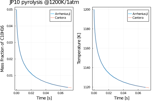
Let us compute the evolution of the mass fractions of C10H16 species as JP-10 is subjected to isobaric pyrolysis at 1 atm and an initial temperature of 1200K. We first include all our packages:
using Arrhenius
using LinearAlgebra
using DifferentialEquations
using ForwardDiff
using DiffEqSensitivity
using Plots
using DelimitedFiles
using Profile
Then create the gas object:
gas = CreateSolution("../../mechanism/JP10skeletal.yaml")Declare the initial conditions as arrays:
Y0 = zeros(ns)
Y0[species_index(gas, "C10H16")] = 0.05
Y0[species_index(gas, "N2")] = 0.95
T0 = 1200.0   #K
P = one_atm
u0 = vcat(Y0, T0);
Create a function to define the ODE problem (for more details on solving differential equations refer to DifferentialEquations.jl.
@inbounds function dudt!(du, u, p, t)
    T = u[end]
    Y = @view(u[1:ns])
    mean_MW = 1. / dot(Y, 1 ./ gas.MW)
    ρ_mass = P / R / T * mean_MW
    X = Y2X(gas, Y, mean_MW)
    C = Y2C(gas, Y, ρ_mass)
    cp_mole, cp_mass = get_cp(gas, T, X, mean_MW)
    h_mole = get_H(gas, T, Y, X)
    S0 = get_S(gas, T, P, X)
    wdot = wdot_func(gas.reaction, T, C, S0, h_mole)
    Ydot = wdot / ρ_mass .* gas.MW
    Tdot = -dot(h_mole, wdot) / ρ_mass / cp_mass
    du .= vcat(Ydot, Tdot)
end
Solve the ODE problem:
tspan = [0.0, 0.07];
prob = ODEProblem(dudt!, u0, tspan);
sol = solve(prob, TRBDF2(), reltol=1e-6, abstol=1e-9);
Great! Let us now compare our solution with cantera by first loading the cantera data:
cantera_data = readdlm("pyrolysis.dat")
ct_ts= cantera_data[:, 1]
ct_T = cantera_data[:, 2]
ct_Y = cantera_data[:, 3:end];
Now plot and compare away:
plt = plot(sol.t, sol[species_index(gas, "C10H16"), :], lw=2, label="Arrhenius.jl");
plot!(plt, ct_ts, ct_Y[:, species_index(gas, "C10H16")], label="Cantera")
ylabel!(plt, "Mass Fraction of C10H16")
xlabel!(plt, "Time [s]")
pltT = plot(sol.t, sol[end, :], lw=2, label="Arrhenius.jl");
plot!(pltT, ct_ts, ct_T, label="Cantera")
ylabel!(pltT, "Temperature [K]")
xlabel!(pltT, "Time [s]")
title!(plt, "JP10 pyrolysis @1200K/1atm")
pltsum = plot(plt, pltT, legend=true, framestyle=:box)
You should get a plot something like this:
Adjoint (Sensitivity) Analysis
In the previous example, we can easily perform a sensitivity analysis using Julia's DiffEqSensitivity.jl:
sensealg = ForwardDiffSensitivity()
alg = TRBDF2()
function fsol(u0)
    sol = solve(prob, u0=u0, alg, tspan = (0.0, 7.e-2),
                reltol=1e-3, abstol=1e-6, sensealg=sensealg)
    return sol[end, end]
end
u0[end] = 1200.0 + rand()
println("timing ode solver ...")
@time fsol(u0)
@time fsol(u0)
@time ForwardDiff.gradient(fsol, u0)
The results are quite promising, with sensitivity computed in less than 2 seconds!
julia>timing ode solver ...
0.405083 seconds (614.32 k allocations: 45.126 MiB)
0.036229 seconds (16.72 k allocations: 11.618 MiB)
1.517267 seconds (183.25 k allocations: 864.085 MiB, 7.46% gc time)
Compute Jacobian using Auto-Diff
Julia's automatic differentiation packages like ForwardDiff.jl can be exploited thoroughly using Arrhenius.jl to compute the Jacobian that frequently pops up while integrating stiff systems in chemically reactive flows. We present to you an example using the LiDryer 9-species H2 combustion mechanism. So let's import packages:
using Arrhenius
using LinearAlgebra
using DifferentialEquations
using ForwardDiff
using DiffEqSensitivity
using Plots
using DelimitedFiles
using Profile
Next input the YAML:
gas = CreateSolution(".../../mechanism/LiDryer.yaml")We use a 9-species + 24-reaction model:
julia> ns = gas.n_species
9
julia> ns = gas.n_species
24
View the participating species:
julia> gas.species_names
9-element Array{String,1}:
 "H2"
 "O2"
 "N2"
 "H"
 "O"
 "OH"
 "HO2"
 "H2O2"
 "H2O"
Let's set the initial conditions:
Y0 = zeros(ns)
Y0[species_index(gas, "H2")] = 0.055463
Y0[species_index(gas, "O2")] = 0.22008
Y0[species_index(gas, "N2")] = 0.724457  #to sum as unity
T0 = 1100.0   #K
P = one_atm * 10.0
u0 = vcat(Y0, T0);
Create the differential function:
function dudt(u)
    T = u[end]
    Y = @view(u[1:ns])
    mean_MW = 1. / dot(Y, 1 ./ gas.MW)
    ρ_mass = P / R / T * mean_MW
    X = Y2X(gas, Y, mean_MW)
    C = Y2C(gas, Y, ρ_mass)
    cp_mole, cp_mass = get_cp(gas, T, X, mean_MW)
    h_mole = get_H(gas, T, Y, X)
    S0 = get_S(gas, T, P, X)
    wdot = wdot_func(gas.reaction, T, C, S0, h_mole)
    Ydot = wdot / ρ_mass .* gas.MW
    Tdot = -dot(h_mole, wdot) / ρ_mass / cp_mass
    du = vcat(Ydot, Tdot)
end
Now computing the jacobian w/ref to the initial condition vector is as simple as:
julia> @time du0 = ForwardDiff.jacobian(dudt, u0)
 0.026856 seconds (18.37 k allocations: 1.047 MiB)
10×10 Array{Float64,2}:
  -0.00227393    -0.000934232   0.000137514  …   0.000213839  -5.21262e-6
  -0.0360919     -0.0148282     0.00218263       0.00334244   -8.27348e-5
   0.0            0.0           0.0              0.0           0.0
   0.00113697     0.000467116  -6.87571e-5      -0.000106919   2.60631e-6
   2.09985e-12    2.28459e-12  -1.26987e-13      2.97389e-12   2.53222e-14
   0.0            0.0           0.0          …   2.74378e-5    0.0
   0.0372289      0.0152953    -0.00225138      -0.00344774    8.53411e-5
   0.0            0.0           0.0              0.0           0.0
   0.0            0.0           0.0             -2.9064e-5     0.0
 -27.3692       -47.4374       16.5061          29.0894       -0.306451
Auto-ignition
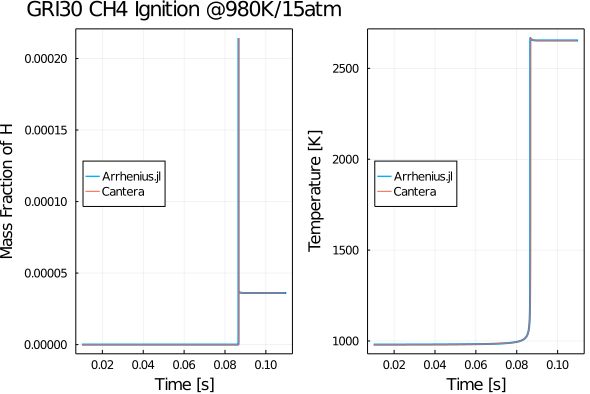
Here we use the GRI30 methane combustion mechanism to compute the ignition delay time of a premixed methane-air mixture @ 980K/15 atm. The implementation is quite similar. Let's say you want to set ICs in-terms of the mole-fractions, one may eventually convert them to mass-fractions as follows:
X0 = zeros(ns);
X0[species_index(gas, "CH4")] = 1.0 / 2.0
X0[species_index(gas, "O2")] = 1.0
X0[species_index(gas, "N2")] = 3.76
X0 = X0 ./ sum(X0);
Y0 = X2Y(gas, X0, dot(X0, gas.MW));
The integrator function remains the same:
u0 = vcat(Y0, T0)
@inbounds function dudt!(du, u, p, t)
    T = u[end]
    Y = @view(u[1:ns])
    mean_MW = 1.0 / dot(Y, 1 ./ gas.MW)
    ρ_mass = P / R / T * mean_MW
    X = Y2X(gas, Y, mean_MW)
    C = Y2C(gas, Y, ρ_mass)
    cp_mole, cp_mass = get_cp(gas, T, X, mean_MW)
    h_mole = get_H(gas, T, Y, X)
    S0 = get_S(gas, T, P, X)
    wdot = wdot_func(gas.reaction, T, C, S0, h_mole)
    Ydot = wdot / ρ_mass .* gas.MW
    Tdot = -dot(h_mole, wdot) / ρ_mass / cp_mass
    du .= vcat(Ydot, Tdot)
end
We then integrate using DifferentialEquations.jl
tspan = [0.0, 0.1];
prob = ODEProblem(dudt!, u0, tspan);
@time sol = solve(prob, CVODE_BDF(), reltol = 1e-6, abstol = 1e-9)
After running ignition.jl you should get a plot as follows:
Global Sensitivity Analysis of Ignition Delay
Coming soon.
Global Sensitivity Analysis of Flame Speed
Coming soon.
Perfect Stirred Reactor
One may refer to the NN-PSR repo
Computational Diagnostic
Coming soon.